Analyzing Rammstein Songs with NLP

Introduction
Disclaimer: I do not own any of the songs and take no responsibility for the content of the mentioned services and websites.
This project analyzes songs produced by the German band Rammstein. What characterizes these songs and how do they compare to each other? will be one question we want to answer. Another one focuses on the change over time, such as did the songs become shorter?
The dataset is has been created by the author. A script constructs the dataset by fetching pieces of the data from
- rammwiki.net: provides list of songs alongside their metadata,
- genius.com: provides a rest API for retrieving song lyrics,
and combines them alongside additional features gained by applying natural language processing techniques via Python. The following python packages have been used to create wordclouds and general preprocessing:
| Package | Usage |
|---|---|
| pandas | Data manipulation |
| requests, beatifulsoup | Web scrapping |
| lyricsgenius | Fetch song lyrics |
| spaCy | Natural Language Processing |
| wordcloud | Create wordclouds |
In addition to Python, the programming language R is used for creating this document and graphs, utilizing the following libraries:
library(dplyr)      # Data manipulation
library(ggplot2)    # Plotting
library(tidytext)   # text processing
library(tidyverse)  # For tidy data
library(tidyr)      # For tidy data
library(ggrepel)    # For annotating graphs
library(lubridate)  # For date parsing/formatting
library(gridExtra)  # Plot arrangement

theme_set(theme_minimal()) # Global ggplot theme
The dataset contains $121$ songs with the folling attributes:
| Attribute | Data type | Description |
|---|---|---|
title | string | Song title |
length | numeric | Duration of the song in seconds |
album | string | The album the song was released with |
release | datetime | Release date of the song |
bpm | numeric | Beats per Minute |
lyrics | string | The annotated song lyrics |
lyrics_cleaned | string | The cleaned lyrics without annotations |
key | string | The key of the song (music theory) |
The dataset contains missing values
| Attribute | title | length | album | release | bpm | key | lyrics | lyrics_cleaned |
|---|---|---|---|---|---|---|---|---|
| # missing | 0 | 1 | 15 | 16 | 25 | 33 | 13 | 15 |
Loading & Preprocessing
The lyrics of each song is quite long, and a preview would be nice, we define a function to truncate the text to a specific length.
truncate_text <- function(text, max_length = 40) {
  if (nchar(text) == 0) return("")
  lines <- unlist(strsplit(text, "\n", fixed = TRUE))
  lines <- lines[sapply(lines, length) > 0]
  short <- lines %>%
    paste(collapse = " ") %>%
    strtrim(max_length) %>%
    paste0("...")
  return(short)
}
data <- read.csv("./data/songs.csv", sep = ";")
Load the dataset and bring the values into the correct format.
Convert the release to a datetime format of YYYY-MM-DD, apply some other formatting of values and add an ID column:
data <- data %>% mutate(
  id = rownames(data),
  title = as.factor(title),
  album = as.factor(album),
  key = as.factor(key),
  release = ymd(release),
  lyrics_preview = sapply(lyrics_cleaned, truncate_text))
Replace indicators for missing values with an empty string "" for qualitative data, and with NaN in case of numeric values.
data$title[data$title == ""] <- NaN
data$length[data$length == 0] <- NaN
data$album[data$album == ""] <- NaN
data$bpm[data$bpm == 0] <- NaN
data$key[data$key == ""] <- NaN
Print summary statistics to get an overview.
summary(data)
        title         length                        album
 5/4       :  1   Min.   :124.0   Liebe ist für alle da:15
 Absinth   :  1   1st Qu.:225.8   Mutter               :13
 Adieu     :  1   Median :249.0   Herzeleid            :11
 Adios     :  1   Mean   :257.0   Rammstein            :11
 Alter Mann:  1   3rd Qu.:284.0   Reise, Reise         :11
 Amerika   :  1   Max.   :720.0   (Other)              :45
 (Other)   :115   NA's   :1       NA's                 :15
    release                bpm             key        lyrics
 Min.   :1994-04-30   Min.   : 38.0   Dm     :27   Length:121
 1st Qu.:1997-11-24   1st Qu.: 78.0   Em     :22   Class :character
 Median :2004-09-27   Median :104.5   Cm     :13   Mode  :character
 Mean   :2006-08-14   Mean   :105.4   D      : 4
 3rd Qu.:2009-10-16   3rd Qu.:130.0   Gm     : 4
 Max.   :2022-04-29   Max.   :190.0   (Other):18
 NA's   :16           NA's   :25      NA's   :33
 lyrics_cleaned          id            lyrics_preview
 Length:121         Length:121         Length:121
 Class :character   Class :character   Class :character
 Mode  :character   Mode  :character   Mode  :character
Inspect Missing Values
How many songs have incomplete data?
incomplete_obs_idx <- apply(data, 1, function(row) sum(is.na(row)) > 0)
num_incomplete_obs <- nrow(data[incomplete_obs_idx, ])
num_total_obs <- nrow(data)
print(paste("Number of songs with missing values:", num_incomplete_obs))
[1] "Number of songs with missing values: 38"
print(paste("Total number of songs:", num_total_obs))
[1] "Total number of songs: 121"
In total 38 of 121 observations have missing values. The columns bpm and release contain the most missing values.
What about the observations with the missing lyrics?
df_missing_lyrics <- data[(data$lyrics == "") | (data$lyrics_cleaned == ""), ]
df_missing_lyrics %>% select(title, length, album, release, bpm, key)
                                          title length      album    release
1                                           5/4    331     Mutter 2002-03-25
2                                       Absinth    236       <NA>       <NA>
12                                      Azzurro    720       <NA>       <NA>
17                                      Claudia    235       <NA>       <NA>
46                                         Holz    297       <NA>       <NA>
47                                      Ich bin    214       <NA>       <NA>
48                                 Ich sehe was    180       <NA>       <NA>
51                                        Intro    124 Völkerball 2006-11-17
59             Lied von der unruhevollen Jugend    293       <NA>       <NA>
94                                 Sonne (1995)     NA       <NA>       <NA>
95                              Sonntag bei Omi    237       <NA>       <NA>
99                                Spring Jungle    203       <NA>       <NA>
100                               Spring weiter    188       <NA>       <NA>
102 Stirb nicht vor mir (Don't Die Before I Do)    245   Rosenrot 2005-10-28
104                                     Student    178       <NA>       <NA>
    bpm  key
1    77    C
2    NA <NA>
12   NA <NA>
17   NA <NA>
46   NA <NA>
47   NA <NA>
48   NA <NA>
51   NA <NA>
59   95    D
94   NA <NA>
95   NA <NA>
99   NA <NA>
100  NA <NA>
102  88   Bm
104  NA <NA>
The above table shows that we know very little about most of the songs.
The songs Intro and Stirb nicht vor mir are also missing other variables.
When researching the two songs on the internet, it turns out that
Introis a live performanceStirb nicht vor miris featuring another artist with english lines.
Therefore we drop all observations shown in above table because they do not add any value to the analysis.
data <- filter(data, !(id %in% df_missing_lyrics$id))
print(paste0("Removed number of songs: ", dim(df_missing_lyrics)[1]))
[1] "Removed number of songs: 15"
print(paste0("Total number of songs: ", dim(data)[1]))
[1] "Total number of songs: 106"
Check the number of missing values for each attribute by defining a helper function.
check_missing_values <- function(df) {
  missing_values_count <- sapply(df, function(row) {
    sum(is.na(row)) + sum(row == "", na.rm = T)
  })
  counts <- unname(missing_values_count)
  feature_names <- names(missing_values_count)
  df_missing <- as.data.frame(t(c("#Missing", counts)))
  colnames(df_missing) <- c("Feature", feature_names)
  return(df_missing)
}
check_missing_values(data)
   Feature title length album release bpm key lyrics lyrics_cleaned id
1 #Missing     0      0     3       4  13  21      0              0  0
  lyrics_preview
1              0
What about the observations with missing release date?
data[is.na(data$release), ] %>%
  select(title, length, release, album, lyrics_preview)
            title length release          album
26      Eisenmann    208    <NA>           <NA>
71         Ramm 4    360    <NA>           <NA>
79 Schwarzes Glas    293    <NA> 6-Track Demo 2
82    Seid bereit    250    <NA>           <NA>
                                lyrics_preview
26 Mein Herz schlägt für Metall Eisen gibt ...
71 Hier kommt die Sonne, das alte Leid Der ...
79 Ein kleiner Wunsch, ach wärt ihr blind W...
82 Hier kommt die Sonne, das alte Leid Der ...
Notice that the album of the songs with unknown release is also unknown.
Looking at the truncated lyrics we can make out that these are legitimate songs.
Imputing the release date does not make sense, but we can replace the missing album values with unknown.
data <- data %>%
  mutate(
    album = as.character(album),
    album = replace(album, is.na(album), "unknown"),
    album = as.factor(album))
We drop the columns key and bpm because we think this data will not contribute any value to the further analysis.
data <- subset(data, select = -c(key, bpm))
data %>% select(-c(id, lyrics, lyrics_cleaned)) %>% head()
       title length        album    release
1      Adieu    278         Zeit 2022-04-29
2      Adios    231       Mutter 2001-04-02
3 Alter Mann    264    Sehnsucht 1997-08-25
4    Amerika    226 Reise, Reise 2004-09-27
5      Amour    290 Reise, Reise 2004-09-27
6      Angst    224         Zeit 2022-04-29
                               lyrics_preview
1 Nur der Tod währt alle Zeit Er flüstert ...
2 Er legt die Nadel auf die Ader Und bitte...
3 Er wartet auf den Mittagswind Die Welle ...
4 We're all living in Amerika Amerika ist ...
5 Die Liebe ist ein wildes Tier Sie atmet ...
6 (Du) (Du) (Du) (Du) (Du) (Du) Wenn die K...
This concludes the data preprocessing. Summarizing we acknowledge the following features with missing data
check_missing_values(data)
   Feature title length album release lyrics lyrics_cleaned id lyrics_preview
1 #Missing     0      0     0       4      0              0  0              0
Inspect Data Distribution
g1 <- ggplot(data, aes(x = length)) +
  geom_boxplot() +
  labs(x = "", y = "") +
  theme(
    axis.text.y.left = element_blank(),
    axis.ticks.y.left = element_blank())
g2 <- ggplot(data, aes(x = length)) +
  geom_histogram(bins = sqrt(nrow(data))) +
  labs(x = "Song duration [s]")
grid.arrange(g1, g2)
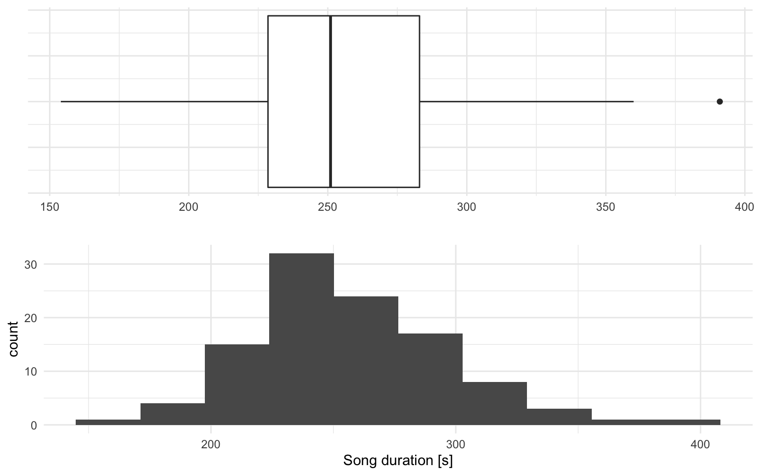
The above boxplot and histogram show an approximately normally distributed data. In order to make sure that we do not have outliers, we investigate the songs with the minimum and maximum duration.
shortest_song <- data[data$length == min(data$length), ]
longest_song <- data[data$length == max(data$length), ]
extreme_songs <- rbind(shortest_song, longest_song)
extreme_songs %>% select(title, length, album, lyrics_preview)
          title length     album                              lyrics_preview
19      Diamant    154 Rammstein Du bist so schön, so wunderschön Ich wil...
67 Pet Sematary    391  Ich will Ok, wir spielen ein Lied für euch und fü...
The two songs seem valid and we keep them in the list.
Finding answers with graphs
Is there seasonality in release dates?
The first plot which might be suitable to answer the question is a time-series plot, binning the release date to year and month and ignoring the day. Unfortunately, this time-series plot results in a busy graph with no clear pattern. To solve the problem, we aggregate the data by month. Sorting the months descending, we can make out the most popular month for releasing songs. The data in question is of categorical (album) and ordinal (number of songs) nature, a dot plot sorted by the number of songs is sufficient for this task.
data %>%
  filter(release != ymd("1994-01-01")) %>%
  mutate(month = month(release, label = TRUE)) %>%
  group_by(month) %>%
  summarise(N = n()) %>%
  ggplot(aes(x = reorder(month, N), y = N)) +
    geom_point() +
    labs(
      title = "Favorite months for releasing songs",
      caption = "Excluding songs with unknown release date.",
      x = "",
      y = "# Songs") +
    coord_flip()
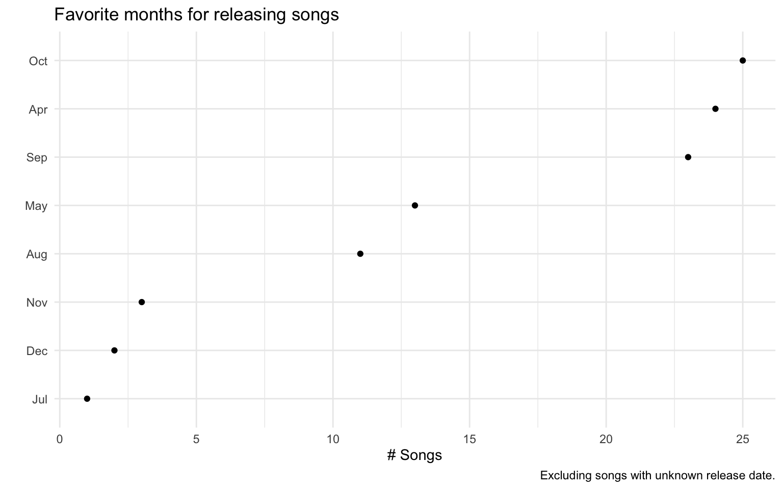
The above plot shows a clear trend: the most popular month for releasing songs are April, September and October. Also August and May are favorite months for releases. We can argue that the band produces songs during the year and publishes them mid-year and mainly at the beginning of autumn.
What characterizes albums regarding the song durations?
First we can check a simple metric: How many songs do the albums contain?
data %>%
  group_by(album) %>%
  summarize(N = n()) %>%
  ggplot(aes(x = reorder(album, N), y = N)) +
    geom_point() +
    labs(x = "", y = "Number of Songs", title = "Number of songs per album") +
    coord_flip()
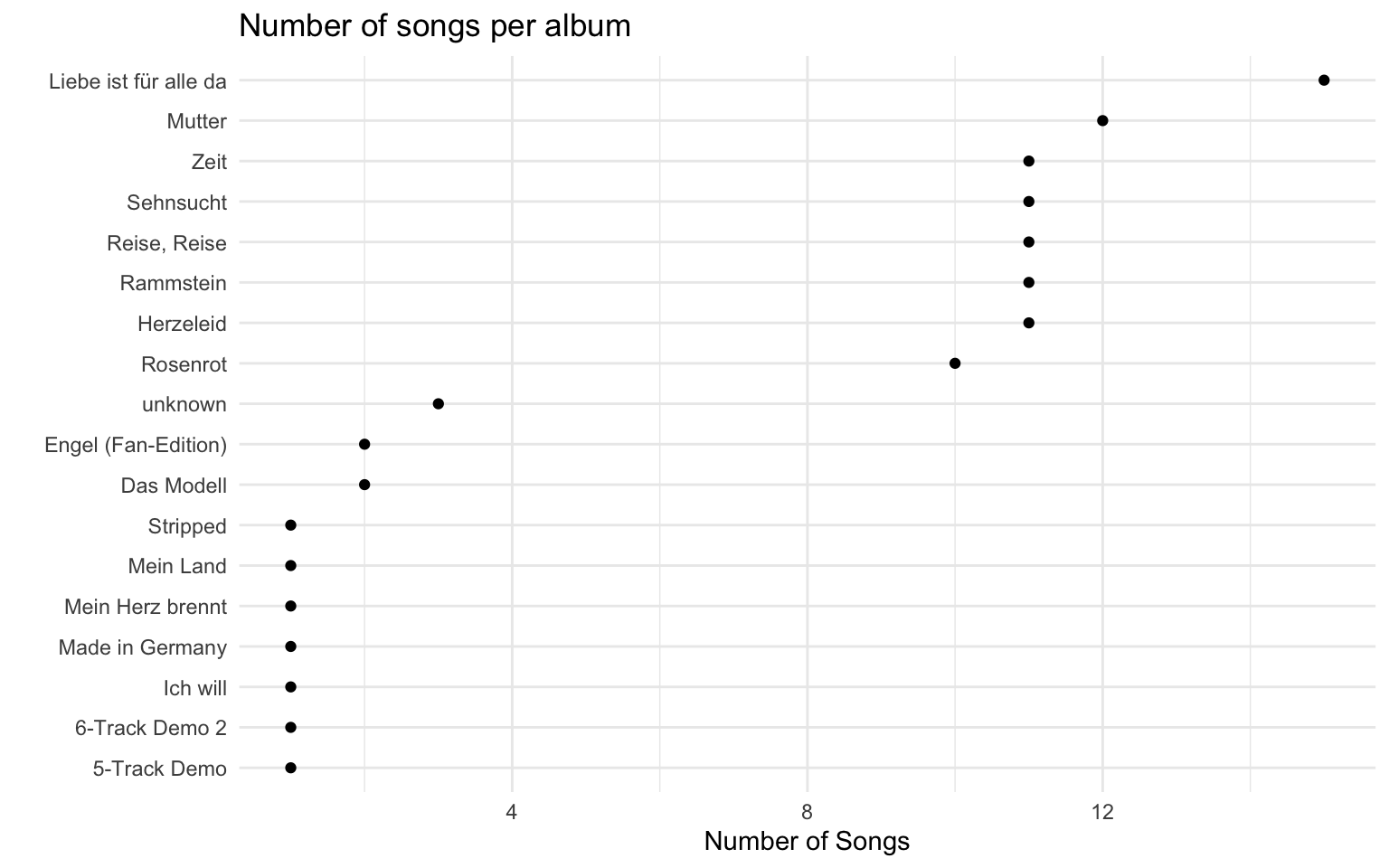
The above plot shows that there are only 8 “real” albums, namely:
- Liebe ist für alle da
- Mutter
- Zeit
- Sehnsucht
- Reise, Reise
- Rammstein
- Herzeleid
- Rosenrot
These are also the officially released albums. We continue the investigation by comparing the song durations of each album over time. When we are mainly interested in the song duration plus confidence interval, per album over time, we have to deal with three components. But a trick allows us to combine the album and time components by concatenating these two pieces of information. Now we have a qualitative ordinal feature (album + release year) and a quantitative feature (mean + confidence interval). The time-representative component is drawn on the x-axis. Utilizing a pointrange geometry for visualizing the quantitative features (mean + confidence interval) we end up with the following figure:
getmode <- function(v) {
   uniqv <- unique(v)
   uniqv[which.max(tabulate(match(v, uniqv)))]
}
data %>%
  mutate(
    year = as.numeric(strftime(release, "%Y")),
    album = paste0(album, "\n", year)) %>%
  group_by(album) %>%
  filter(n() > 5) %>%
  summarize(
    year = getmode(year),
    mean_length = mean(length),
    stddev_length = sd(length)) %>%
  ungroup() %>%
  ggplot(aes(x = reorder(album, year), y = mean_length)) +
    geom_pointrange(aes(
      ymin = mean_length - stddev_length,
      ymax = mean_length + stddev_length)) +
    labs(x = "", y = "Mean song duration [s] with confidence range",
      title = "Comparing song durations per album over time",
      caption = "Considering only official albums.") +
    theme(axis.text.x = element_text(size = 7))
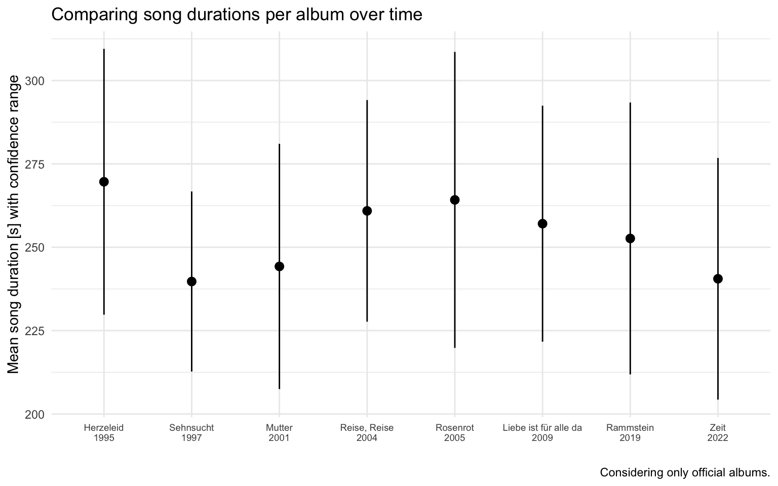
The above plot shows a clear trend towards shorter songs. In retrospective a boxplot could have worked too, but we actively decided against because it makes the figure busy.
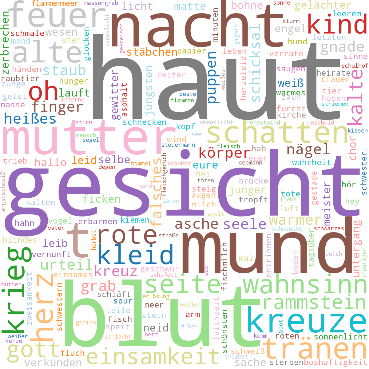
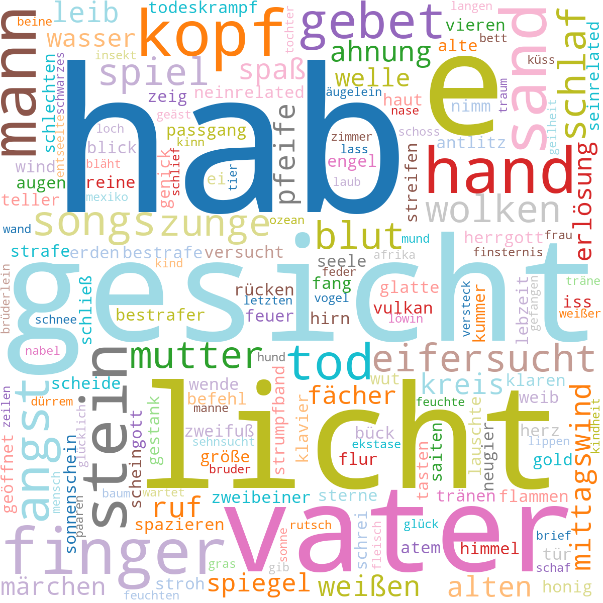
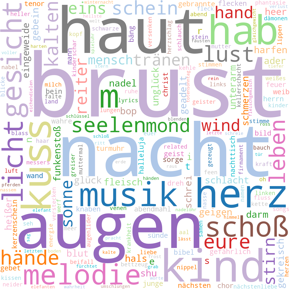
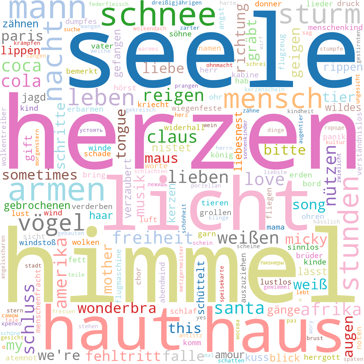
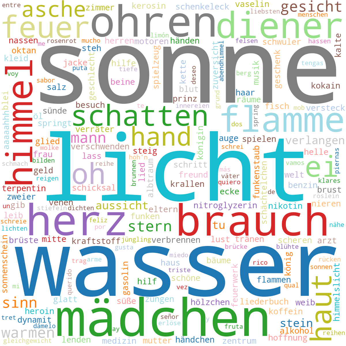
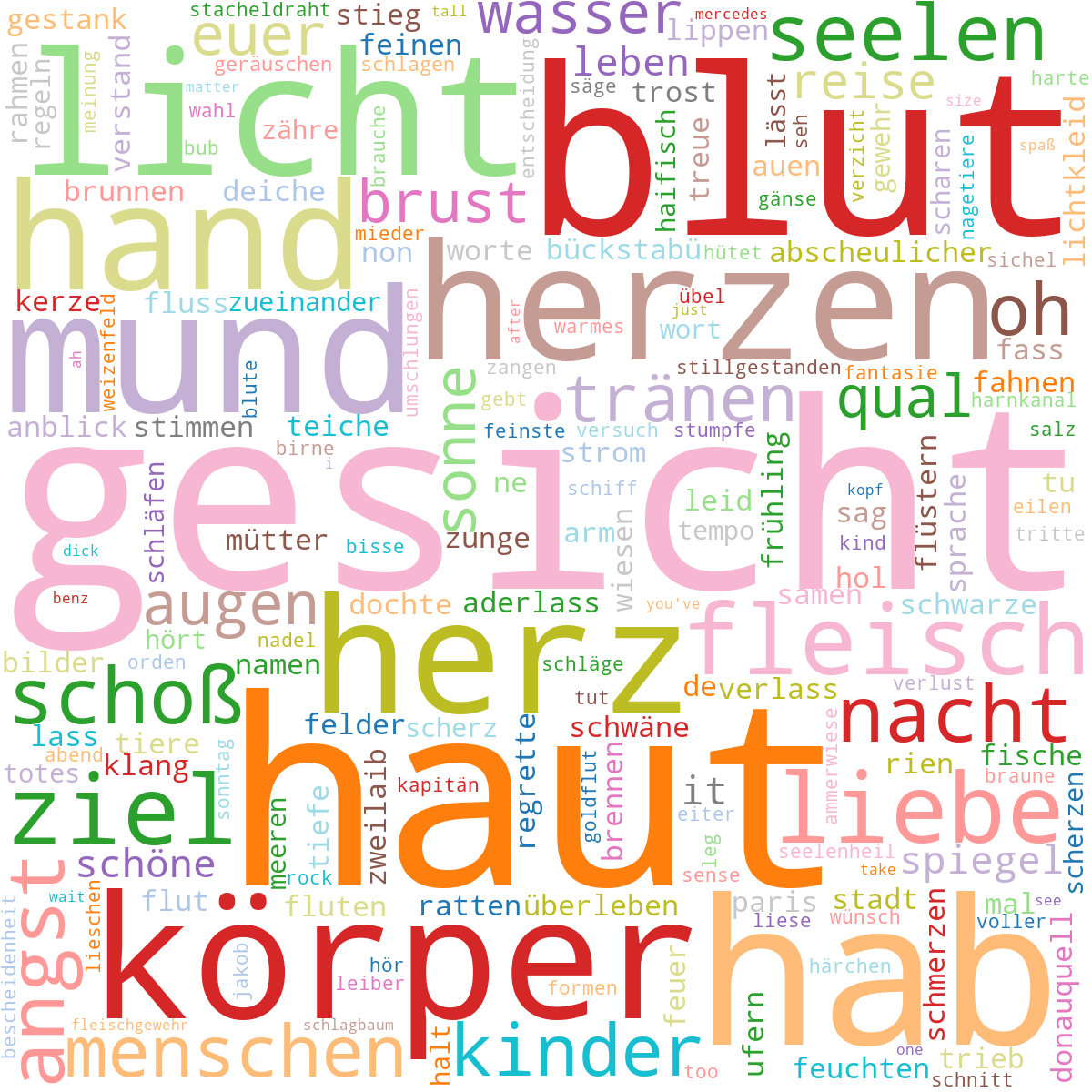
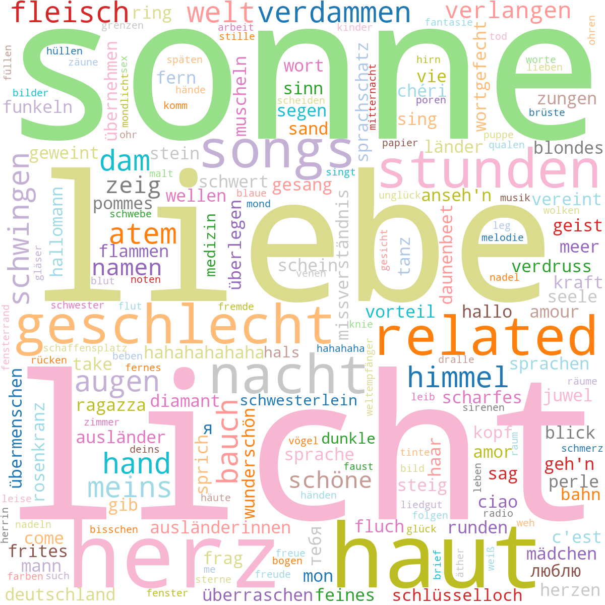
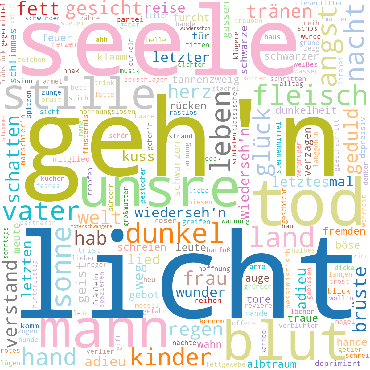
What characterizes the album content?
How can we compare the album contents (text), how do they differ?
Word clouds provide a wunderful way to summarize the contents of each album.
A pipeline implemented in Python which utilizes the spaCy natural language processing package processes the lyrics by applying tokenization, lemmatization and part-of-speech (PoS) tagging.
Considering only specific tokens such as nouns or adjectives, we can paint a clear picture summarizing the album content with a few words.
Some songs heavily repeat words, therefore only consider the unique words of every song.
Differentiating between qualitative data requires a qualitative color map.
 |  |
 |  |
 |  |
 |  |
Peter W. Egger
Software Engineer / Data Scientist
Maker culture enthusiast and aspiring data scientist.