Classify hand gesture sEMG data with neural networks
Introduction
The dataset used in this project is surface EMG data collected with the Myo armband from Thalmic Labs and is available at kaggle.com, provided by [1]. The device is mounted on the arm and sensor readings have been captured while performing the following gestures:
index_fingermiddle_fingerring_ringerlittle_fingerthumbrestvictory_gesture
The sensor has eight electrodes from which measurements have been recorded. Therefore the question we want to solve in this report is to classify the measurements into one of the above classes.
The dataset contains several types of data:
- raw, unprocessed data,
- cropped and arranged data,
- data with extracted features; this applies advanced algorithms to characterize the motion data.
The author has left no documentation on how the data has been captured, opening up questions like:
- What type of sensor/electrode has been used?
- Where was the sensor attached, what is the exact position on the arm?
- Was the data captured on only one user, or several?
- What is the granularity of the data, was it measured each $ms$, $\mu s$?
- The metadata for the raw data is missing, leaving us in the dark on what the data represents: is this a measurement of a single gesture, or multiple ones right after one another?
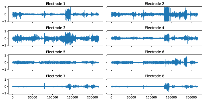
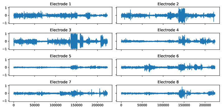
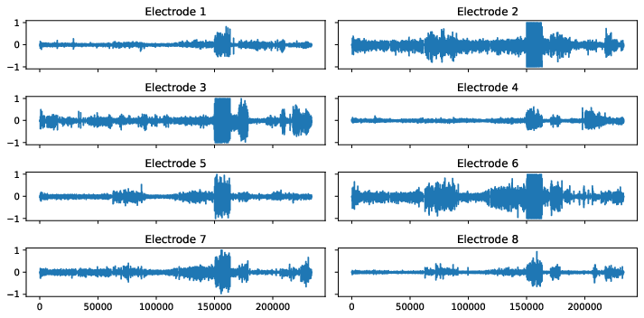
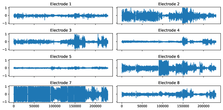
The below figures visualize the raw data for each gesture. Note that the rest_finger gesture is not completely flat for some electrodes.
 |  |
 |  |
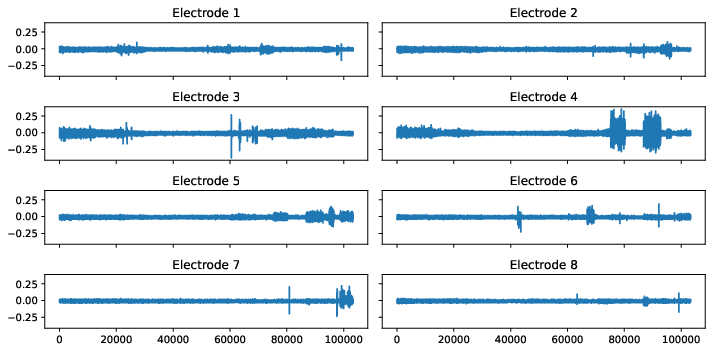 | 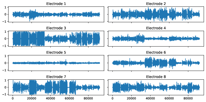 |
Figure 1: Sensor readings for several hand gestures.
As mentioned above there is no detailed documentation about the raw data, therefore we work with the preprocessed data which extracted the following features:
| Feature | Variable Name |
|---|---|
| Standard deviation | stdev |
| Root mean square | root_mean_square |
| Minimum | min |
| Maximum | max |
| Zero crossing | zero_crossing |
| Average amplitude change | avg_amplitude_change |
| First birst of amplitude | amplitude_first_burst |
| Mean absolute value | mean_absolute_value |
| Waveform length | wave_form_length |
| Wilson (or Willison) amplitude | willison_amplitude |
Table 1: List of extracted features from the raw data.
The exact definition of the above statistics are explained in Feature reduction and selection for EMG signal classification [2].
The preprocessed data is presented in the following form
| Feature | 0 | 1 | 2 | 3 | 4 |
|---|---|---|---|---|---|
e0_stdev | $0.029437$ | $0.035060$ | $0.043982$ | $0.032677$ | $0.032101$ |
e1_stdev | $0.051465$ | $0.025699$ | $0.033187$ | $0.031038$ | $0.029580$ |
e2_stdev | $0.089432$ | $0.025286$ | $0.071985$ | $0.033345$ | $0.035939$ |
e3_stdev | $0.016893$ | $0.020039$ | $0.018900$ | $0.020213$ | $0.037279$ |
e4_stdev | $0.014127$ | $0.012505$ | $0.016712$ | $0.016290$ | $0.014564$ |
| $\cdots$ | $\cdots$ | $\cdots$ | $\cdots$ | $\cdots$ | $\cdots$ |
e4_willison_amplitude | $0.000000$ | $0.000000$ | $1.000000$ | $0.000000$ | $0.000000$ |
e5_willison_amplitude | $1.000000$ | $0.000000$ | $2.000000$ | $2.000000$ | $1.000000$ |
e6_willison_amplitude | $1.000000$ | $1.000000$ | $1.000000$ | $2.000000$ | $0.000000$ |
e7_willison_amplitude | $0.000000$ | $1.000000$ | $2.000000$ | $1.000000$ | $0.000000$ |
class | 1 | 1 | 1 | 1 |
Table 2: Examples for preprocessed data.
where the prefixes $e0, e1, \ldots, e7$ indicate the corresponding electrode from which the measurement has been taken. The dataset has $6823$ records with $80$ features. The class mapping is given by the following table
| Label | Encoded Label |
|---|---|
index_finger | 1 |
middle_finger | 2 |
ring_ringer | 3 |
little_finger | 4 |
thumb | 5 |
rest | 6 |
victory_gesture | 7 |
Table 3: Label encoding table.
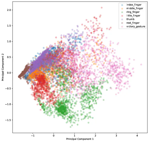
To get a feeling for the data we visualize the first two components of the principal component analysis.
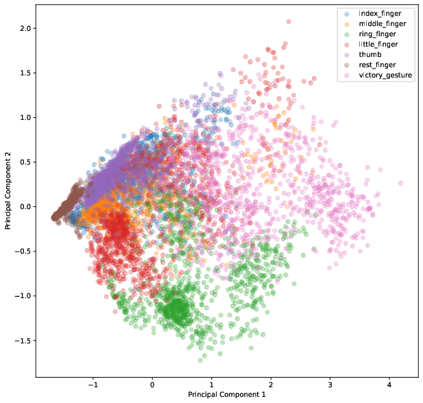
The result of the PCA is illustrated in Figure 2 and shows that especially the classes index_finger, middle_finger and thumb have many overlapping observations.
This indicates that the classes might be difficult to separate because they share some common structure. Thinking about the anatomy of the body it could mean that the same muscles are utilized when pointing with one of those fingers.
As we will see later in the conclusion, the suspicion is verified by the model’s performance.
Model Architecture
Inspiration for the ANN architecture is drawn from the article Latent Factors Limiting the Performance of sEMG-Interfaces [3] which uses a feed-forward network with a single hidden layer containing eight neurons – using the sigmoid function as activation.
Tests showed that using the sigmoid activation function generally yields better results than ReLu or TanH for this specific problem. Furthermore, the sigmoid function improved the training speed by converging faster to an accuracy of around $80%$, whereas the other activation functions resulted in oscillations and slow learning.
As there are seven different classes to predict, stating a multiclass-classification problem, the output layer consists of seven neurons activated by the softmax function.
Several architectures have been tried out, starting at one hidden-layer networks to two hidden layers with varying amount of neurons. Concluding with the result that a single hidden layer containing around $16$ neurons produces the best result. Anything lesser than this amount of neurons results in underfitting, and adding more neurons ends in overfitting where the model does not learn the necessary abstract structure of the data. Preventing overfitting with a dropout layer did not proof to be useful as it triggered oscillations in the learning curve and resulted in worse results than without. An early stopping criteria monitoring the loss function is used in the code to prevent overfitting during training.
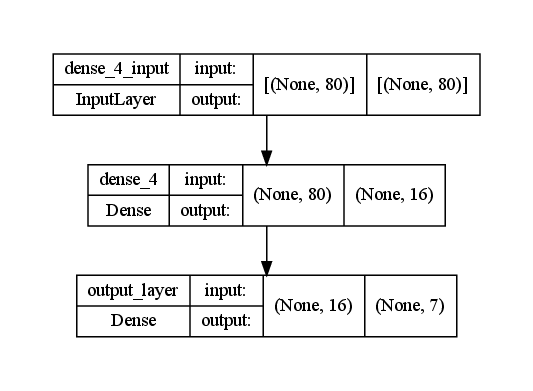
Data preprocessing is not necessary, except for reshaping the target variable from a one-dimensional array into a two-dimensional one in order to comply with the model architecture (which has an output neuron for each class). This is done by one-hot encoding the target variable:
| Label | One-hot encoded label |
|---|---|
| $1$ | $[1, 0, 0, 0, 0, 0, 0]$ |
| $2$ | $[0, 1, 0, 0, 0, 0, 0]$ |
| $3$ | $[0, 0, 1, 0, 0, 0, 0]$ |
| $4$ | $[0, 0, 0, 1, 0, 0, 0]$ |
| $5$ | $[0, 0, 0, 0, 1, 0, 0]$ |
| $6$ | $[0, 0, 0, 0, 0, 1, 0]$ |
| $7$ | $[0, 0, 0, 0, 0, 0, 1]$ |
Table 4: One-hot encoding the target variable to comply with the model architecture.
Training Results
The data is split into training and validation set with a test size of $33%$. The training data is fed into the the network with a batch size of $16$, a validation split of $0.25$ and $200$ epochs.
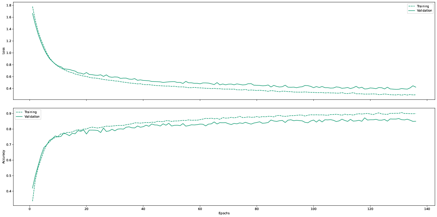
Starting at around epoch $50$, the training and validation loss/accuracy start to slightly diverge and continue almost parallel, as depicted in Figure 4. This marks the point to stop the training and save the model.
We can evaluate the model performance by using sklearn’s performance_report method and the previously splitted test data which is completely unknown to the model:
| Precision | Recall | F1-Score | Support | |
|---|---|---|---|---|
| index_finger | $0.69$ | $0.70$ | $0.70$ | $343$ |
| middle_finger | $0.88$ | $0.75$ | $0.81$ | $336$ |
| ring_finger | $0.88$ | $0.96$ | $0.92$ | $345$ |
| little_finger | $0.77$ | $0.78$ | $0.78$ | $358$ |
| thumb | $0.76$ | $0.74$ | $0.75$ | $335$ |
| rest_finger | $0.97$ | $0.98$ | $0.97$ | $240$ |
| victory_gesture | $0.89$ | $0.95$ | $0.92$ | $295$ |
| accuracy | $0.83$ | $2252$ | ||
| macro avg | $0.84$ | $0.84$ | $0.84$ | $2252$ |
| weighted avg | $0.83$ | $0.83$ | $0.83$ | $2252$ |
Table 5: Output of the performance report.
The Table 5 shows overall good results of an average accuracy of around $80%$. Predictions of the classes rest_finger, ring_finger and victory_gesture yield are more accurate.
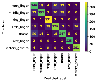
The suspision of misclassification of the thumb, index and middle finger classes is supported by the results of Figure 5.
The confusion matrix reflects the results of the principal component analysis where it is difficult to differentiate those classes. For example, thumb is often predicted as index_finger, which is shown in Figure 2 by the overlapping observations.
Conclusion
There are many methods available for preprocessing EMG data as listed by Feature reduction and selection for EMG signal classification [2] and are common practice to use. Metadata is very important to get a good understanding of the data and know how to work with it. It was quite interesing to use the results from the principal component analysis (see Figure 2) to explain the model behaviour (see misclassifications in Figure 5). Alltogether, the model presented in this paper performs quite well, but it can definitely be improved by further investigating preprocessing methods to better separate the problematic classes, or even adapt the model architecture to solve this problem. This is also described as a problem in Latent Factors Limiting the Performance of sEMG-Interfaces [3] which compares two models (ANN and LDA) and concludes that the model performance is equally good but is influenced by factors impacting the sensor itself, such as the body fat index and other characteristics of the test subjects.
References
[1] https://www.kaggle.com/nccvector, “Electromyography(EMG) dataset.” 2019 [Online]. Available: https://www.kaggle.com/datasets/nccvector/electromyography-emg-dataset
[2] A. Phinyomark, P. Phukpattaranont, and C. Limsakul, “Feature reduction and selection for EMG signal classification,” Expert Systems with Applications, vol. 39, no. 8, pp. 7420–7431, Jun. 2012, doi: 10.1016/j.eswa.2012.01.102.
[3] S. Lobov, N. Krilova, I. Kastalskiy, V. Kazantsev, and V. Makarov, “Latent Factors Limiting the Performance of sEMG-Interfaces,” Sensors, vol. 18, no. 4, p. 1122, Apr. 2018, doi: 10.3390/s18041122.
Peter W. Egger
Software Engineer / Data Scientist
Maker culture enthusiast and aspiring data scientist.